Optimization refers to the process of minimizing or maximizing the objective function f(x) that consists of the variable x. In machine learning or deep learning terminology, it is usually meant to minimize the loss function J(w), where the model parameter w∈R^d. The minimization optimization algorithm has the following goals:
- If the objective function is convex, then any local minimum is a global minimum.
- Normally, in most deep learning problems, the objective function is non-convex. It can only find the lowest value in the neighborhood of the objective function.
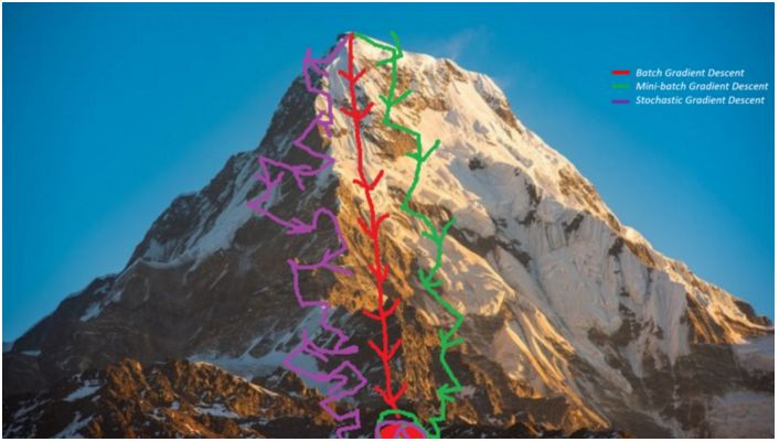
Figure 1: Moving towards Minimization
There are currently three main optimization algorithms:
- For single point problems, the optimization algorithm does not require iteration and simple solution.
- Gradient descent method is often used in logistic regression. This type of optimization algorithm is essentially iterative, and it can converge to an acceptable solution regardless of the parameter initialization.
- For a series of problems with non-convex loss functions, such as neural networks. To ensure convergence speed and low error rate, parameter initialization in the optimization algorithm plays a crucial role.
Gradient descent is the most commonly used optimization algorithm in machine learning and deep learning. It belongs to the first-order optimization algorithm. Only the first-order derivative is considered when the parameters are updated. In each iteration, the gradient represents the steepest rising direction, so we update the parameters in the opposite direction of the gradient of the objective function and adjust the step to reach the local minimum in each iteration by learning the rate α. Therefore, the objective function will go downhill until it reaches a local minimum.
In this article, we will introduce the gradient descent algorithm and its variants: batch gradient descent, small batch gradient descent, and stochastic gradient descent.
Let's first look at how gradient descent works in logistic regression, and then discuss other variant algorithms. For simplicity, we assume that the logistic regression model has only two parameters: the weight w and the deviation b.
1. Set initialization weight w and deviation b to any random number.
2. Choose a suitable value for the learning rate α. The learning rate determines the step size for each iteration.
- If α is very small, it takes a long time to converge and the amount of calculation is large.
- If α is large, it may not be possible to converge or even exceed the minimum value.
- Through us we will use the following values ​​as learning speed: 0.001, 0.003, 0.01, 0.03, 0.1, 0.3.
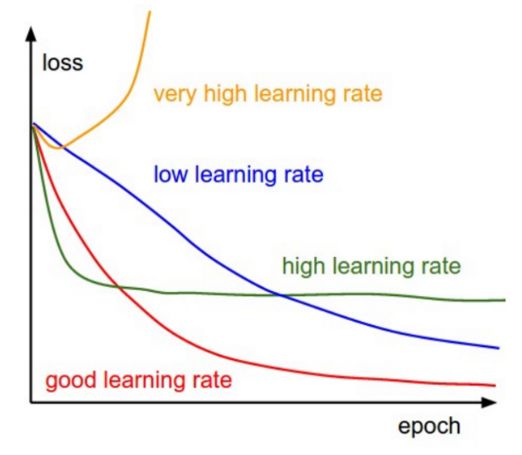
Figure 2: Gradient descent at different learning speeds
Therefore, by observing and comparing the loss function changes corresponding to different alpha values, we choose the first one that does not reach the converged alpha value as the final alpha value, so that we can have a fast and convergent learning algorithm.
3. If the data scale is different, scale the data. If we do not scale the data, the contours (contours) will become narrower and narrower, meaning that it takes longer to reach convergence (see Figure 3).
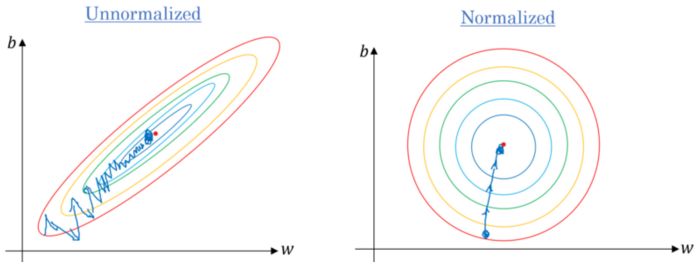
Figure 3. Gradient Descent: Normalized vs. Contoured vs. Unnormalized Data
Make the data distribution satisfy μ = 0 and σ = 1. The following is the data scaling formula:

4. In each iteration, use the partial derivative of the loss function J to represent each parameter (gradient)

The updated equation is as follows:

- Specifically, here we assume that there is no deviation. If the gradient direction corresponding to the current value w is positive, which means that the current point is on the right side of the optimal value w*, then it needs to be updated toward the negative direction so as to approach the optimal value w*. However, if the gradient is now negative, the update direction will be positive and will increase the current value of w to converge to the optimal value of w* (see Figure 4):
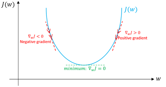
Figure 4: Gradient descent, illustrating how the gradient descent algorithm uses the first derivative of the loss function to achieve a descent and reach a minimum.
- Continue this process until the loss function converges. That is, until the error curve becomes flat.
- In addition, each iteration moves in the direction of greatest change, each step being perpendicular to the contour.
The above is the general process of the gradient descent method. We need to determine the objective function, optimization method, and guide the system to find the optimal value through the gradient.
Now we discuss three variants of the gradient descent algorithm. The main difference between them is the amount of data used to calculate the gradient in each learning step, which is the gradient accuracy and time complexity for each parameter update (learning step). Eclectic considerations.
Batch gradient drop
Bulk gradient descent means that all samples are used in each iteration when updates are performed on the parameters.

For i in range(num_epochs):
Grad = compute_gradient(data, params)
Params = params — learning_rate * grad
The main advantages:
- During training, we can use a fixed learning rate, regardless of the attenuation of the learning rate.
- It has a linear trajectory towards the minimum value, and if the loss function is convex, it guarantees theoretical convergence to a global minimum, and if the loss function is not convex, it converges to a local minimum.
- The gradient is unbiased. The more samples, the lower the standard error.
The main shortcomings:
- Although we can use vector calculations, it may still be slow to traverse all samples, especially when the data set is large, the algorithm time will become a serious problem.
- Each step in the learning process involves traversing all the samples. Some of the samples may be redundant and do not contribute much to the update.
Small batches of gradient drops
In order to overcome the shortcomings of the above methods, people have proposed a small batch of gradients. When updating each parameter, instead of traversing all the samples, only a part of the samples is used for updating. Therefore, each time only the small batches of b samples are used for updating learning, the main process is as follows:

- Disturb training datasets to avoid pre-existing sequential structures of samples.
- The training data set is divided into b small batches according to the size of the batch. If the training set size cannot be divisible by the batch size, the remaining portion is used as a small batch.
For i in range(num_epochs):
Np.random.shuffle(data)
For batch in radom_minibatches(data, batch_size=32):
Grad = compute_gradient(batch, params)
Params = params — learning_rate * grad
The size of the batch we can adjust, usually chosen as the power of 2, for example 32,64,128,256,512 and so on. The reason behind this is that some hardware like GPU is also getting a better run time with a power-of-two batch size.
The main advantages:
- Faster than batch gradients, because it uses less samples.
- Randomly selecting samples helps to avoid interference that does not contribute much to the learning of redundant samples or very similar samples.
- When the size of the batch is smaller than the size of the training set, it will increase the noise during the learning process and help to improve the generalization error.
- Although more standard samples can be used to obtain lower estimated standard errors, the computational burden is less than linear growth
The main drawbacks:
- In each iteration, the learning step may move back and forth due to noise. Therefore it fluctuates around the minimum area but does not converge.
- Due to noise, there will be more oscillations in the learning steps (see Figure 4), and as we get closer to the minimum, we need to increase the learning attenuation to reduce the learning rate.
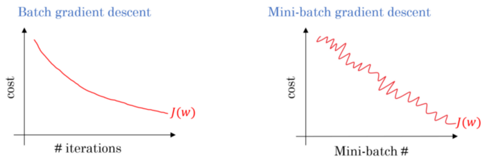
Figure 5: Gradient Descent: Comparison of Loss Functions for Bulk and Small Lots
For large-scale training data sets, we usually do not need more than 2-10 times to traverse all the training samples. Note: When the batch size b is equal to the number of training samples m, this method is equivalent to a decrease in the batch gradient.
Stochastic gradient descent
Stochastic gradient descent (SGD) only performs parameter updates on samples (xi, yi) instead of traversing all the samples. Therefore, learning occurs on each sample. The specific process is as follows:

- Disturb training data sets to avoid sample pre-existing order
- Divide the training data set into m samples.
For i in range(num_epochs):
Np.random.shuffle(data)
For example in data:
Grad = compute_gradient(example, params)
Params = params — learning_rate * grad
It has many similar advantages and disadvantages with the small batch version. The following are features specific to SGD:
- Compared with the small batch method, it adds more noise to the learning process and helps to improve the generalization error. However, it also increases the running time.
- We cannot process 1 sample in the form of a vector, leading to very slow speeds. In addition, because we use only 1 sample for each learning step, the variance will increase.
The following figure shows the gradient descent variants and their direction towards the minimum value. As shown in the figure, the direction of the SGD is noisy compared to the low-volume version:
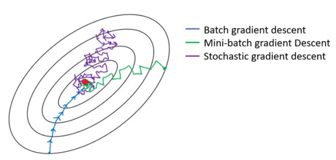
Figure 6: Trajectory of the gradient descent variant towards the minimum
difficulty
The following are some of the common problems encountered with gradient descent algorithms and their variants:
- The gradient descent is a first-order optimization algorithm, which means that it does not consider the second derivative of the loss function. However, the curvature of the function affects the size of each learning step. The gradient describes the steepness of the curve, and the second derivative measures the curvature of the curve. So if:
1. Second derivative = 0 → The curvature is linear. Therefore, the step length = learning rate α.
2. Second derivative > 0 → curvature upward. Therefore, the step size <learning rate α may cause divergence.
3. Second derivative <0 → curvature down. Therefore, the step > learning rate α.
Therefore, the direction that seems promising for the gradient may not be the same, and may result in slowing or even divergence of the learning process.
- If the Hessian matrix is ​​not good enough, for example, the direction of the maximum curvature is much larger than the curvature of the direction of the minimum curvature. This will cause the loss function to be very sensitive in some directions and insensitive in other directions. Therefore, some directions that seem to favor the gradient may not cause the loss function to change significantly (see Figure 7).
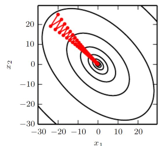
Figure 7: The gradient descent fails to exploit the curvature information contained in the Hessian matrix.
- As each learning step is completed, the norm of the gradient gTg should slowly decrease as the curve becomes more flat and the steepness of the curve decreases. However, the norm of the gradient is increasing due to the curvature of the curve. Despite this, we were able to obtain a very low error rate (see Figure 8).
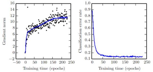
Figure 8: Gradient Norm. Source
- In small-scale data sets, local minimums are common; however, saddle points are more common in large-scale data sets. Saddle point refers to a function that bends upward in some directions and downward in other directions. In other words, the saddle point looks like a minimum in one direction and a maximum in the other direction (see Figure 9). This happens when at least one of the Hessian matrix eigenvalues ​​is negative and the rest of the eigenvalues ​​are positive.
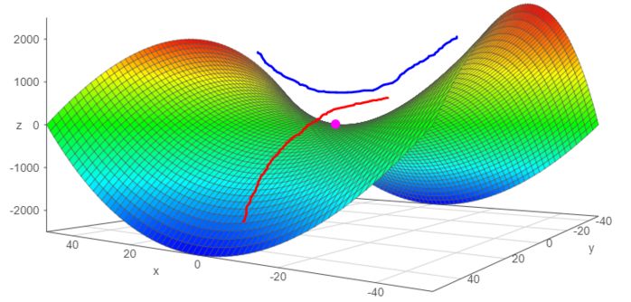
Figure 9: Saddle Point
- As mentioned earlier, it is difficult to choose the appropriate learning rate. In addition, for small batch gradients, we must adjust the learning rate during training to ensure that it converges to a local minimum rather than wandering around it. It is also difficult to calculate the decay rate of the learning rate, and this will vary with the data set.
- All parameter updates have the same learning rate; however, we may prefer to perform a larger update on some of the parameters, because the directional derivatives of these parameters are closer to the minimum trajectory than the other parameters, then the targeted setting is needed. Learning rate and its changes.
We are the largest supplier of RELX in China. High quality 100% Original supply, wholesale price is reasonable
It only takes 7-15 days from China to the destination, with a full range of flavors and styles.
RELX disposable electronic cigarettes, devices and pods. The latest factory date and the most complete supply chain
Relx Infinity Case vape E-Cigarette Device Vape Pod wholesale
Suitable for:
All>18
Atomizing Concentration:
Low
Nic Content:
None
Flavor:
Fruits Series
Puffs:Vape 600 Puffs
Relx Infinity Pod
Disposable:
Disposable
Basic Info.
Model NO.
relx Infinity pod
Name
Relx Vape Pod
Tank Capacity
1.8ml Capacity Relx Vape pod
MOQ
100PCS
Rechargeable Vape
Yes
Compatible
Veex & Sp2s & Vapemoho Mini
Transport Package
10 pieces in a large box
Trademark
veex cartridge
Origin
China
Product Description
High quality 1.8ml vape pod RELX infinity pod relx cartridge
Relx infinity Pod Specifications :
Pod Capacity:
1.8ml
Wicking Material:
FEELM Cotton Wicking Material
Pod Weight:
6g
Pod Life Span:
Vape 600 Puffs


Relx Vape,Relx Disposable Vape 600 puffs,RELX Guava flavor Pod,Relx Vape Kit infinity,Diverse style Relx Vape Kit
Tsvape E-cigarette Supplier Wholesale/OEM/ODM , https://www.tsvaping.com